↜ Back to index Introduction to Numerical Analysis 1
Part b—Lecture 5
In today’s lecture we implement the numerical method for the wave equation.
Implementation of the finite difference scheme
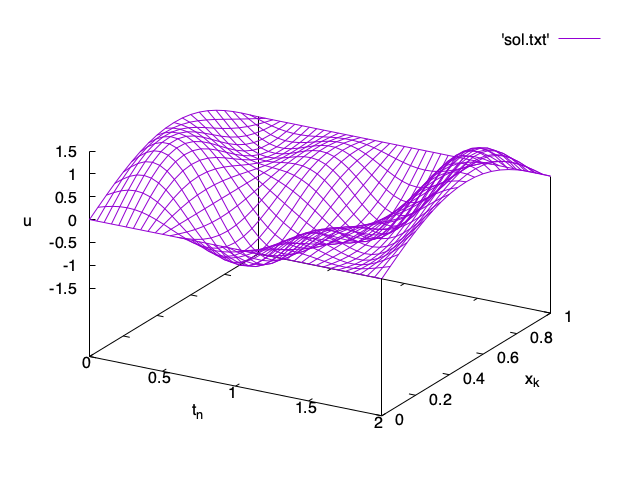
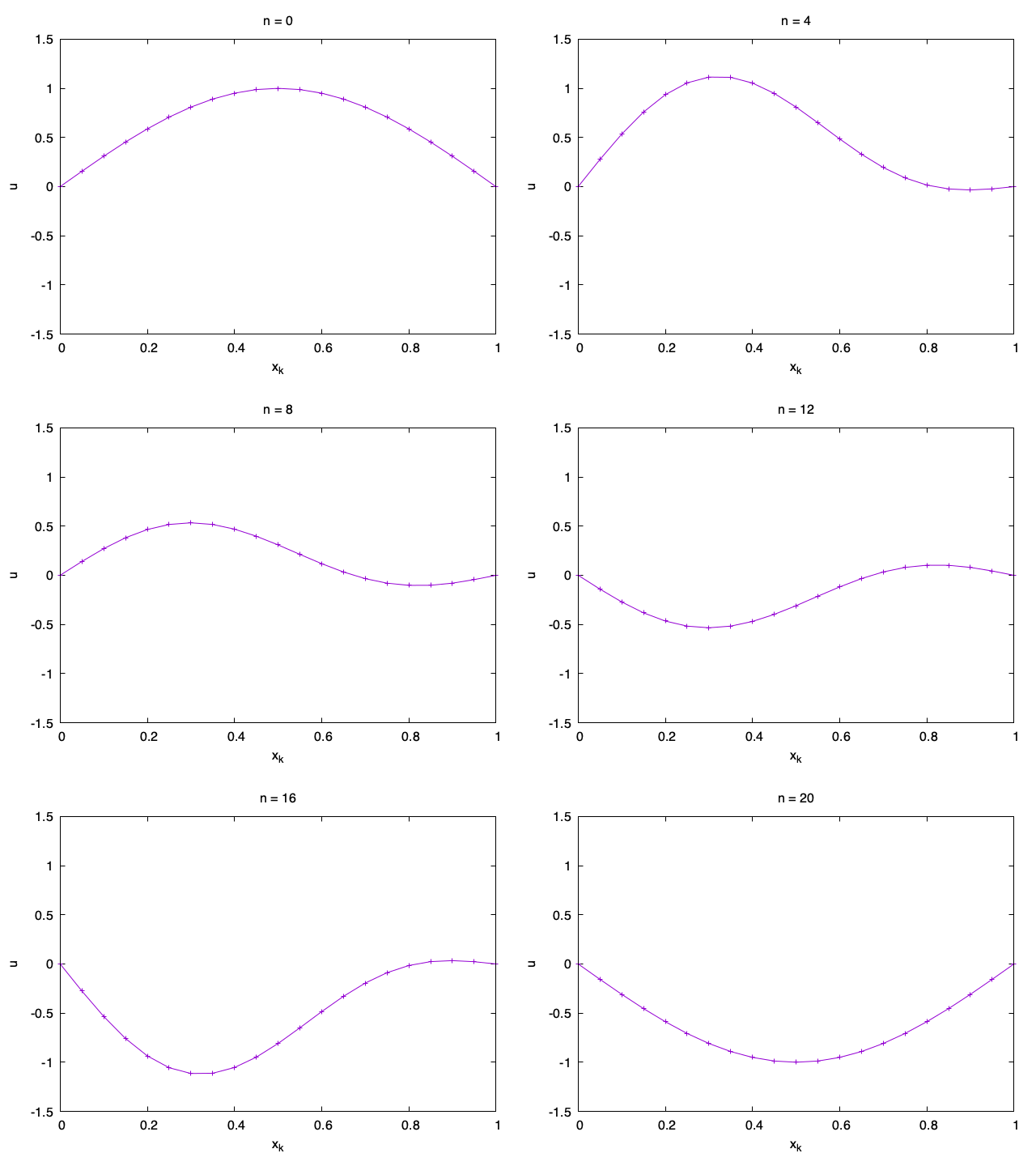
Here is an example Fortran code for the case a = b = 0 and u_0(x) = \sin(\pi x), v_0(x) = \pi \sin(2\pi x), M = 20 and \tau = h.
implicit none
! introduce constants M and pi
integer, parameter :: M = 20
real, parameter :: pi = 4. * atan(1.)
integer n, k, nmax
real h, tau, x, r
! We need three arrays to store n-1 (uprev), n (u) and n+1 (w) steps
real, dimension(0:M) :: u, uprev, w

h = 1. / M
tau = h
!      👇 we solve the problem up to time t_nmax = 2.
nmax = 2. / tau
r = tau**2 / h**2

! Initialize uprev with the initial data u_0 and print the values.
! Since sin(0) = sin(pi) = 0 = a = b, we do not need to set the boundary data
! separately.
do k=0, M
    x = k * h
    uprev(k) = sin(pi * x)
    print *, 0., x, uprev(k)
end do
! Print an empty line (needed for gnuplot)
print *

! Now we compute u_{1,k} (values at n = 1) and store them in u
u(0) = uprev(0)     ! boundary condition is constant
print *, tau, 0, u(0)
do k=1, M-1
    x = k * h
    !                       /-----------------\ this is v_0
    u(k) = uprev(k) + tau * pi * sin(2 * pi * x) &
         + 0.5 * r * (uprev(k-1) - 2 * uprev(k) + uprev(k + 1))
    print *, tau, x, u(k)
end do
u(M) = uprev(M)
print *, tau, 1., u(M)
! Print an empty line (needed for gnuplot)
print *

! The main loop
do n=1, nmax-1
    ! One step of the finite difference method from u_n to u_{n+1}
    ! Array u holds the values of u_n, uprev the values of u_{n-1}.
    ! Array w will be filled with computed values of u_{n+1}.

    w(0) = u(0) ! boundary condition is constant in time
    do k = 1, M-1
        w(k) = 2 * u(k) - uprev(k) + r * (u(k - 1) - 2 * u(k) + u(k + 1))
    end do
    w(M) = u(M) ! boundary condition is constant in time

    ! print the values of the solution at t_{n+1}
    do k = 0, M
        print *, (n + 1) * tau, k * h, w(k)
    end do
    ! print an empty line (needed for gnuplot)
    print *

    ! store the values of v in u and u in uprev; the order is important!
    uprev = u
    u = w
end do
end
Note that we can now take timestep \tau = h. This is much larger than the timestep \tau = h^2 / 4 that we had to take for the heat equation due to the stability condition discussed in Lecture b3. The finite difference scheme for the wave equation has a much weaker condition.
Stability condition for the scheme for the wave equation.
\tau \leq h
The output of the program consists of values t_n, x_k and u_{n, k}, one (n, k) per line. There is an empty line between blocks of values with different n so that gnuplot understands the data as being on a two-dimensional grid.
   0.00000000       0.00000000       0.00000000
   0.00000000       5.00000007E-02  0.156434476
   0.00000000      0.100000001      0.309017003
   0.00000000      0.150000006      0.453990549
   0.00000000      0.200000003      0.587785244
   0.00000000      0.250000000      0.707106829
   0.00000000      0.300000012      0.809017062
   0.00000000      0.349999994      0.891006529
   0.00000000      0.400000006      0.951056540
   0.00000000      0.450000018      0.987688363
   0.00000000      0.500000000       1.00000000
   0.00000000      0.550000012      0.987688303
   0.00000000      0.600000024      0.951056480
   0.00000000      0.650000036      0.891006470
   0.00000000      0.699999988      0.809017003
   0.00000000      0.750000000      0.707106769
   0.00000000      0.800000012      0.587785184
   0.00000000      0.850000024      0.453990370
   0.00000000      0.900000036      0.309016794
   0.00000000      0.949999988      0.156434447
   0.00000000       1.00000000      -8.74227766E-08

   5.00000007E-02           0   0.00000000
   5.00000007E-02   5.00000007E-02  0.203048781
   5.00000007E-02  0.100000001      0.397541583
   ...
We can plot the data using gnuplot’s splot command as in the case of the heat equation.

However, it is often easier to understand what is happening by making a movie with graphs of the solution u_{n, k} as a function of x_k one n at a time.

Exercise 1. Modify the Fortran code and solve the wave equation on domain x \in (0,1), t \in (0, 2) for each of the following data:
- u_0(x) = x(2 - x), v_0(x) = 1, a = 0, b = 1
- u_0(x) = \frac 12 - |x- \frac 12|, v_0(x) = 0, a = b = 0
- u_0(x) = H(x - \frac 12), v_0(x) = 0, a = 0, b = 1, where H(s) = 1 for s \geq 0 and H(s) = 0 for s < 0.
Plot the numerical solutions in gnuplot.
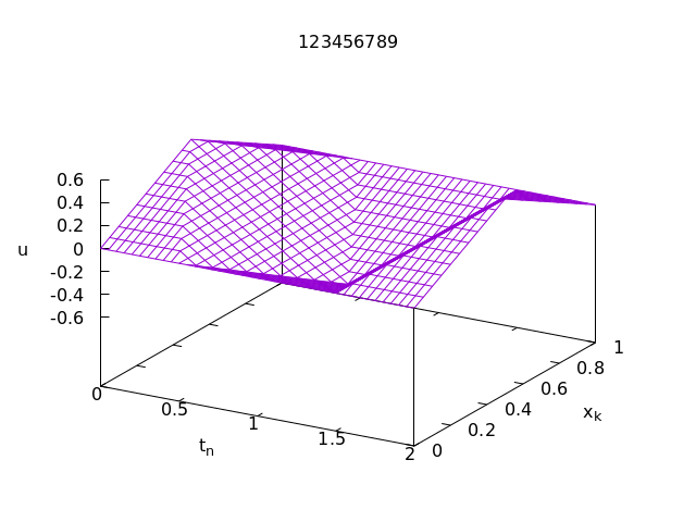
Submit the plot for 2. with M = 20 and \tau = h to LMS with your student ID as the title.
Example solutions
Exercise 1-2.
The submitted plot should look something like this:

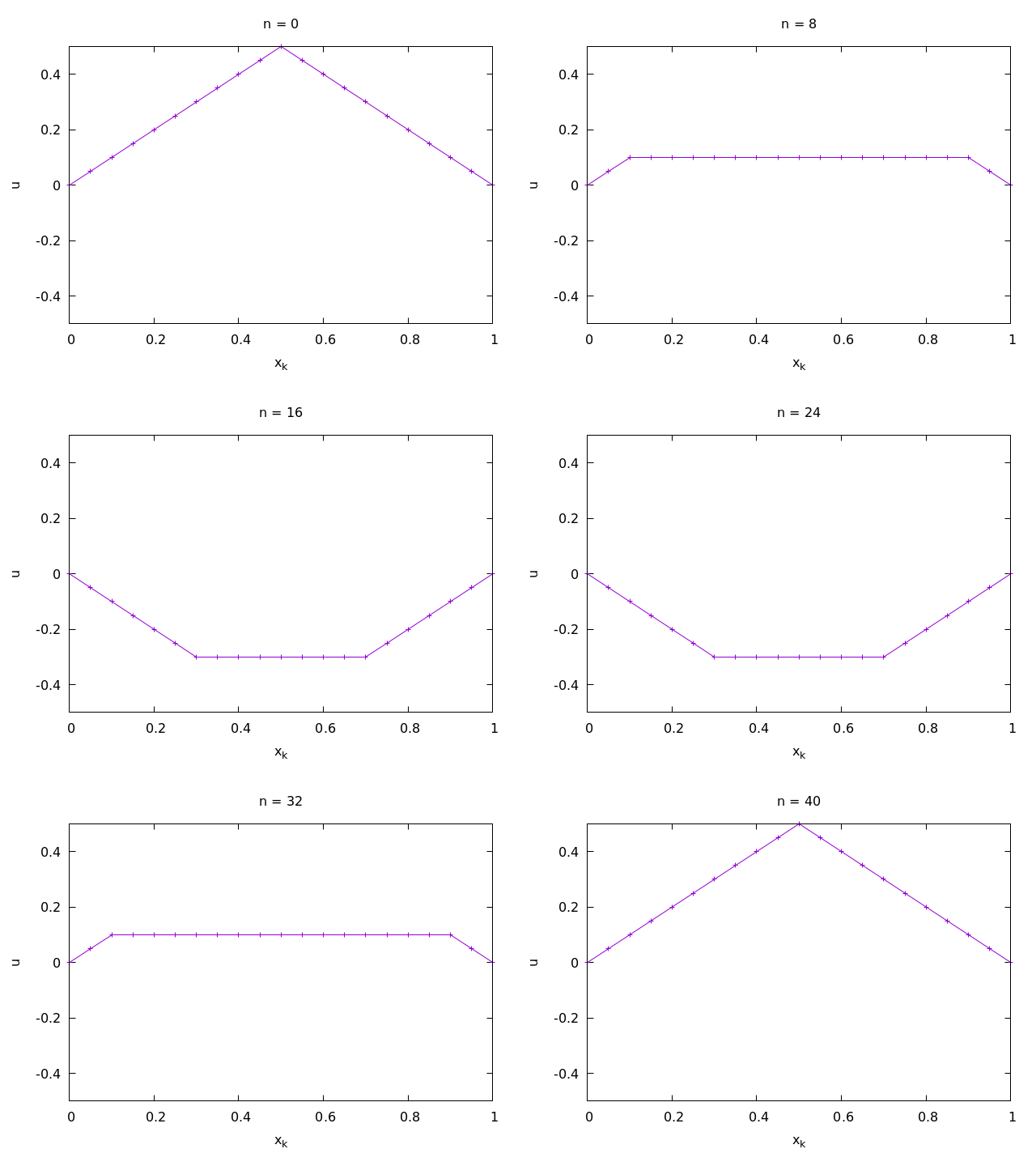
This is an animation of the above solutions (not visible in the pdf note):

When looking at the numerical solution, you should notice that it is not a differential function. In what sense is it then a solution of the wave equation, which requires second derivatives? We can consider even nondifferentiable functions as solutions of partial differential equations in some generalized sense (weak sense): for example in the sense of distributions. You will learn about this in advanced classes on PDEs.